Global Physics Settings
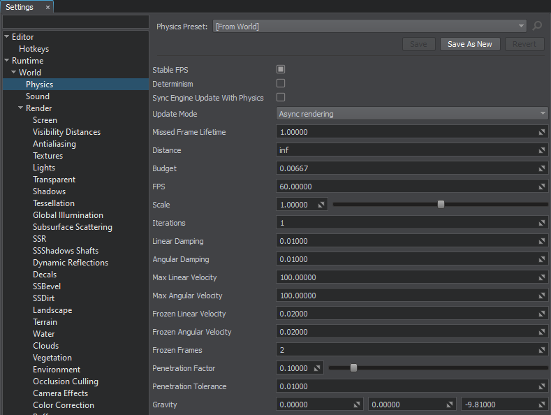
The Physics section of the Settings window allows you to adjust global physics-related settings: values set here will be applied to all physical objects in the scene.
For more information on how to add physical properties to objects and set up physical interactions, see the articles in the Physics section.

The following settings are available:
| Stable FPS |
Toggles frame time stabilization on and off. In case the current Engine framerate is much higher than the fixed Physics framerate (e.g. 120 FPS vs 60 FPS), the physics won't be updated each rendering frame (e.g. it may update during every second frame). The resulting frame time will become unstable, shorter-longer-shorter-longer (render -> render+physics -> render -> render+physics...). This option ensures stable frame time for smoother user experience removing unwanted "hiccups" (however, the average framerate is decreased). Notice
By default, this option is enabled. But you can disable it to increase average framerate in case the application is used for machine learning or for grabbing frame sequences (Video Grabber), when smoothness is not important. |
||
|---|---|---|---|
| Determinism |
Toggles Deterministic mode on and off. Deterministic mode ensures that all contacts are solved in the predefined order and visualization of physics in the world is repetitive (on one computer). When this mode is enabled, the Engine performs additional sorting of bodies, shapes, and joints inside islands after building them. Notice
|
||
| Sync Engine Update With Physics |
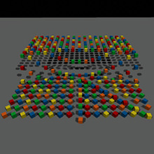
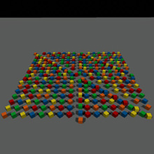
Toggles synchronization of the Engine FPS with the physics one. Such FPS limitation makes it possible to calculate physics each rendered frame (rather then interpolate it when this option is disabled). In this mode, there is no twitching of physical objects if they have non-linear velocities. If the Engine FPS is lower than the physics one, this option has no effect. |
||
| Update Mode |
Update mode to be used for physics:
|
||
| Missed Frame Lifetime | Lifetime for missed frames, in milliseconds. This value defines how long missed frames are to be kept in the catch-up buffer. In case the current Engine framerate is lower than the fixed Physics framerate, some of the physics frames get skipped and the simulation starts looking like in a slo-mo effect (e.g., if the target physics framerate is 60 FPS, when the Engine updates at 30 FPS, the simulation will look 2 times slower). The Physics module will try to catch up everything missed later, when possible (e.g. when the Engine framerate grows higher, while waiting for GPU to complete rendering). The missed frames are kept in a buffer for some time (lifetime), as it expires the frame is removed from the buffer and becomes lost forever. Notice
Setting too high values may result in significant memory consumption in case of low hardware capabilities (no catching-up performed with a growing number of missed frames). |
||
| Distance | Distance from the camera, from which physical interactions will not be calculated. All physics-based nodes freeze if the distance between them and the camera is bigger than the Physics distance. The distance is measured from the camera to the node's bound.
|
||
| Budget | Physics simulation time budget in seconds. | ||
| FPS | Fixed frame rate used to simulate physics. Physics frame rate is independent of the rendering one.
Notice
If physics takes more than the assigned time budget, further calculations are delayed. These calculations shall be performed during the subsequent rendering frames, making physics simulation look like in a "slo-mo" mode. The default budget is 50 ms, but it can be increased, as necessary. |
||
| Scale | Scale factor to speed up or slow down the physics simulation time, i.e how frequently physics is simulated (for example, slowing down of body's velocity). Only physics ticks are affected, while everything else is rendered at a normal speed. | ||
| Iterations | The number of iterations for physics during one physics tick. Each iteration the full cycle of physics simulation is performed:
Notice
High number of iterations increases stability, but also results in a higher load. If physics takes more than set in the time budget, next iterations are automatically delayed and moved to the next rendering frame. |
||
| Linear damp | Damping of objects' linear velocities. This value is added to the linear damping set individually for each object.
|
||
| Angular damp | Damping of objects' angular velocities. This value is added to the angular damping set individually for each object.
|
||
| Max linear velocity | The maximum possible linear velocity.
|
||
| Max angular velocity | The maximum possible angular velocity.
|
||
| Frozen linear velocity | Linear velocity at which the object becomes frozen, if it keeps both of its velocities (angular and linear) lower than the freeze velocities.
|
||
| Frozen angular velocity | Angular velocity at which the object becomes frozen, if it keeps both of its velocities (angular and linear) lower than the freeze velocities.
|
||
| Frozen frames | The number of frames, during which an object should keep both its angular and linear velocities under the specified level to become frozen. | ||
| Penetration factor | The factor used to define the rebounding force in case of penetration.
|
||
| Penetration tolerance | Distance in units indicating how deep one object can penetrate another to be rebounded. | ||
| Gravity | Three coordinates of the vector used to define a gravity. It creates a world-wide uniform force field. Gravity is applied at the center of mass of each body (except for dummy body) to calculate its acceleration.
|
Watch an overview of the global physics settings in our video tutorial on physics.

